Faceted search is a vital part of LinkedIn’s search experience. It’s a key feature in the exploratory searches done by job seekers, recruiters and market analysts when trying to find the information they need on LinkedIn. It provides structure to search results, which enables fast navigation and discovery.

When it comes to a great search experience, there are two elements that matter most: correctness and performance. Conventional approaches to faceted search sacrifice either too much correctness or don’t perform fast enough.

This post covers a new approach to faceted search based on inverted index, this is compared to the conventional forward index-based approach. We outline technical challenges and superiority of the new approach when dealing with very large data sets. We also include some practical results from the largest LinkedIn search index to back up our ideas. It is important to note that this post assumes a basic familiarity with the inverted index-based approaches to search.

What is faceted search?

Faceted search is best explained through an example. In the screenshot below, there are two facets, 'Location' and 'Current Company', each with multiple facet values. Some facet values like 'LinkedIn', 'Greater New York City Area' and 'San Francisco Bay Area' are selected. If the original query was 'Software Engineer', the facet selections mean the actual results include software engineers from the New York City Area or the Bay Area and who work at LinkedIn.

In the above example, the astute reader would have noticed that multiple facet value selections within the same facet are treated as an OR, i.e. the selections for 'Location' indicate we want engineers in New York City OR the Bay Area. The counts reflect these semantics: a selection of a facet value within a facet like 'Location' will not affect the counts of other locations. If this were not true, the counts of all other locations would become 0 once we select a location like 'San Francisco Bay Area'. This is not very useful or intuitive.

The challenges of faceted search

The LinkedIn search stack, called Galene, supports early termination by providing features like static rank along with special retrieval queries (which we will discuss in future posts). Early termination enables us to do typeahead searches using an inverted index, and enables queries with lots of hits to execute fast. For example, in typeahead we index two-letter prefixes, which match millions of documents per shard. There is no cost-effective way to provide millisecond latencies for those queries if we were to retrieve and score all documents.

On the other hand, early termination doesn't work well with the standard approach for faceting. The standard way to discover facet values and compute their counts is to use forward index while scoring documents. Facet values are put in priority queues and several facet values with highest counts are selected to ultimately be displayed on the search page left rail.

If we terminate a search without retrieving all documents, we will have inaccurate counts for low cardinality facet values if we use this forward index based approach. This challenge is compounded if we want to estimate the counts of high cardinality facet values through some sort of sampling.

In summary, doing facet counting using the forward index means that we cannot do two things at the same time:

• Approximate facet counts for large cardinality facet values to improve performance
• Guarantee exact values for low counts

The last requirement is very important as typically when count is low (something which fits on a couple of search pages) the numbers should be exact while discrepancies in high numbers don't matter too much, i.e. it doesn't matter if we have 10200 or 10215 results, but it matters if we have 5 or 6 results.

Our solution

Thus we had to come up with a different algorithm for faceting. We chose to use inverted index posting lists to count facet values. Using the inverted index for facet counting allows us to guarantee exact counts for low cardinality, while at the same time allowing us to estimate the counts for high cardinality values, providing a significant performance boost. Our approach also retains the option for us to early terminate when scoring documents.

First, we split the faceted search problem into two components: discovery and counting. Facet discovery is the process of deciding which values to display for a given facet. For example, the 'Current Company' facet requires us to 'discover' a list of companies that we are going to display. This list is based on the input query, so the companies shown for the query 'Software Engineer' will be different from the companies shown for the query 'Mechanical Engineer'.

Our decision was to use forward index to discover facet values during scoring and to use the inverted index to count them. These two steps are sequential as counting can't start until at least some facet values are discovered.

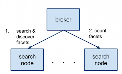
The typical search cluster setup consists of multiple index partitions hosted on search nodes and a broker, which does a fan-out request and gathers results. When faceting is involved, the broker typically does two requests: the first one performs regular scoring and discovers facet values along the way. Once the broker gathers all facets values the search nodes it issues a subsequent request to count the top N values for each facet.

Facet discovery

When using early termination search query is typically augmented to retrieve most relevant documents while skipping non-relevant ones. This way, facet values from non-relevant documents might be skipped during the retrieval stage or they can be discarded during top N selection on broker, which introduces relevance component into the way we select facet values to display.

The problem arises when a facet selection is made. In this case we can not use search query to discover facets as facet selection becomes a part of it while it should not be considered during discovery of a selected facet.

Let's say we have facet value LinkedIn selected for Current Company facet. Let's also say that our early termination limit is 100 and we need at least 50 documents to discover facets. Essentially we need to execute the following queries:

1. (+Engineer +LinkedIn) [100]
2. +Engineer [50]

• '+' means that a clause is required. When having two or more clauses it can be thought as boolean AND.
• [100] and [50] are early termination limits

Query 1 will be used for scoring as well as for discovery of facets other than Current Company. Query 2 will be used for discovery of Current Company facet. It's possible to multiplex these two queries into a single one:

1. (+Engineer ?LinkedIn[100]) [50]

• '?' means that a clause is optional. When having two or more clauses it can be thought as boolean OR. In this case it's combined with a required clause, so it becomes fully optional, meaning it doesn't have to match at all.
• [100] means early termination limit on ?LinkedIn clause.

The query above retrieves same documents as two separate queries but doing it much more efficiently in a single pass. The necessity of multiplexing becomes evident when having two or more facets selected. Fortunately similar logic can be applied in this case as well.

Using the inverted index for facet counting

To use the inverted index for facet counting, we created a special counting query which can be executed like any other query that utilizes the posting lists of the inverted index. For example, the following query will count the engineers in Google, Facebook and LinkedIn by essentially traversing the posting lists for the terms 'Engineer', 'Google', 'Facebook', and 'LinkedIn':

FACETS Google Facebook LinkedIn QUERY Engineer

The result of this query will be a set of (facet value, facet count) pairs. QUERY means the original query issued by a user, in this case 'Engineer', and is called the query condition. When counting, each search node essentially executes the following query:

+Engineer +(?Google ?Facebook ?LinkedIn)

This query matches only documents which contribute to at least one facet value count. For each matched document, we increment the count of the corresponding facet value. Since we have an 'OR' expression, each matched document can increment multiple facet value counts.

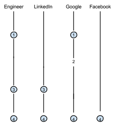
Consider the example above. It shows an inverted index with 4 terms and 4 documents with docids 1 - 4. The circled docids indicate that the counting query produced a match.

The first document matches query condition and it also matches 'Google'. The second document matches only 'Google' and will not be counted. The third document matches the query condition and 'LinkedIn'. The fourth document matches everything. The counting query will match documents 1, 3, and 4. After counting is finished it will produce the following counts: Google 2, Facebook 1, LinkedIn 2.

When facet values are selected, the facet counting query becomes more complicated. But it still can be constructed and executed in a single pass similar to the above, matching only those documents which contribute to at least one facet value count.

Counting approximation

The approach above is correct, but will result in poor performance for queries which match millions of documents per shard.

It is here where the use of the inverted index pays dividends: since the inverted index posting lists come with skip lists, we can leverage this to sample a subset of the index and produce estimated counts for large cardinalities.

When using sampling, the counting query can be rewritten to:

+Engineer 
+(
    ?(+Google +Google_Sampling) 
    ?(+Facebook +Facebook_Sampling) 
    ?(+LinkedIn +LinkedIn_Sampling) 
    ?Engineer_Sampling
)

There are many ways to implement sampling iterator. We've experimented with quite a few different approaches, but the following one is quite performant and provides very good accuracy in the same time.

The idea is to compute facet value count as:

where D(x) is a facet value density function. It's a continuous function defined on [0,max doc] and takes values in a range [0, 1].

For performance sake we use linear interpolation to approximate D(x), which provides decent enough accuracy. We split document id space into R equal ranges of size S = max doc / R. Sampling iterator then returns up to F first documents from each range. As document id space is contiguous the implementation of the sampling iterator boils down to several arithmetic operations. We then calculate density value D(x) for the beginning of each range r as M(r) / F, where M(r) is amount of documents matched against corresponding facet value iterator in a range r. Finally we integrate density function D(x) to compute facet count:

Since this approach actually retrieves documents from the entire posting list, it works very well regardless of the distribution of documents. This is important because we have observed that our static rank tends to make posting lists dense at the front and sparse at the end, e.g. a posting list with document ids 1, 2, 4, 6, 20, 100, 1000 can be very typical.

Example

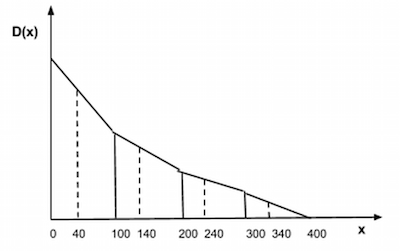
Let's say we have document ids in 0-400 range. We split them into R = 4 equal intervals, 100 documents each. We consider 40 first documents from each interval to compute density function D(x).

Let's say that:

1. first interval matched 10 documents with facet count iterator
2. second - 5 documents
3. third - 2 documents
4. fourth - 1 document

We calculate square under function D(x) by evaluating 400/2/40/4*(10 + 5 + 5 + 2 + 2 + 1 + 1 + 0) = 32.5

This way the final approximated count is reported to be 33.

Results

The following study was done based on a query logs from the main member search product on LinkedIn. We applied our approximation algorithm for each query and compared results against the algorithm with approximations turned off.

• Capacity: total runtime decreased by a factor of 7
• Latencies: p50 decreased 1.2 times, p90 - 1.4 times, p95 - 2.6 times, p99 - 11.5 times

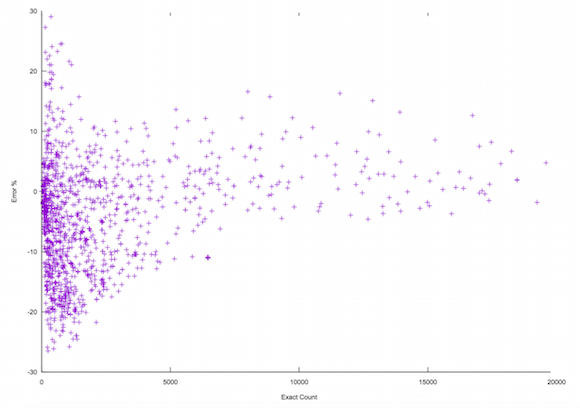
This plot above displays percentage of error for the estimated counts. X is the exact count we would get if not using any approximations. Y axis is the percentage error of the approximation. The plot shows that our error is never more than 30% with p95 = 5% and p99 = 17% It's important to realize that approximations start only upon configured threshold (45 in the plot above) so the error rate for exact count less than 45 is guaranteed to be 0%.

Conclusion

To summarize, our goal with the new faceting was threefold:

• To retain the the option of early terminating searches when the result set is large.
• To guarantee exact counts for low cardinality facet values.
• To improve the performance of counting large facet values by providing estimated counts.

We achieved these goals by splitting the faceting operation into two separate phases: discovery and counting. We used the traditional forward index scan approach for discovery, and used an inverted index traversal with sampling for the counting phase. With this approach we were able to achieve the right balance of correctness and performance.

Results show tremendous gains in capacity and high percentile latencies. The key to this approach is the flexibility it provides to tune different knobs to make different tradeoffs between correctness and performance.

Acknowledgements

Many thanks to search infrastructure engineers, who worked on faceting, especially Apurva Mehta, Niranjan Balasubramanian, Yingchao Liu, Choongsoon Jesse Chang and Michael Chernyak.