Making Your Feed More Relevant – Part 2: Relevance models and features

This is a follow up post to Making Your Feed More Relevantthat provided introductory background on the feed system at LinkedIn. In this post we will dive deep into relevance models and features.

We use many metrics for assessing the engagement level that the feed provides. Below are a few such metrics:

• Interactions: number of clicks, likes, comments, follows, joins, connects, re-shares
• Viral actions: number of likes, comments, and re-shares
• Shares: number of re-shares
• Engaged feed sessions: number of sessions in which the user either scrolled down the feed to view at least 10 updates, or interacted with a feed item.

These metrics can be per-user (divided by the total number of users), or overall. Interactions per-user is abbreviated as CTR (click through rate). Metrics that capture immediate reaction to the feed are called upstream metrics (for example interactions or CTR) while metrics that capture delayed reaction to the feed are called downstream metrics (for example, engaged feed sessions).

It is much easier to predict and optimize upstream metrics than downstream metrics. The feed relevance model is trained to predict the interaction rate associated with the viewer and specific updates. That model is used to construct the personalized feed. Specifically, the model performs the following actions:

1. Estimates the probability that the viewer will interact with each update P (interaction = yes | viewer, update) (we refer to this as the predicted CTR of the update or pCTR).
2. Create an initial ranked list of updates by ranking updates according to their pCTR.
3. Create the final list by reranking the initial list.

In this blog post we focus on task 1 above. Task 2 is a simple task of ordering updates by their scores, and task 3 is described in the next blog post in this series.

Probabilistic Model

We abbreviate the interaction of user i on update t by the binary variable  (1 if there is an interaction and -1 otherwise). Our modeling assumption is that  follows a logistic regression model (conditional on the viewer and update), which is a standard assumption in the industry. Specifically, assuming that is a vector of parameters capturing the model and is a vector of features characterizing the viewer, the update, and the context, the logistic regression model is

,

which is equivalent to

.

The parameter vector specifies the model, and is learned during the training stage by maximizing the likelihood of the training data.

Training data

We collect training data for some fixed time period from a random bucket (a set of users that receive feed updates that are a random shuffle of the top-k updates as ranked by the current SPR^[1]). Specifically, we collect response variables  for all users and all updates that were served to the users, together with the associated feature vectors . The updates with which a viewer interacted with (=1) are considered positive examples and those with which the viewer did not interact with (=0) are treated as negative examples.

Model training

The parameter vector  is selected by maximizing the likelihood of the training data as a function of 

.

Such likelihood maximization modeling techniques have been used for decades in statistics and are still standard practice in the industry.

More specifically, the maximization is done as follows:

1. Form the loglikelihood function that is the log of the likelihood function above and that is easier to maximize. The maximizer of the loglikelihood is also guaranteed to be the maximizer of the likelihood function.
2. Add a regularization term (Euclidean norm on the parameter vector) to the loglikelihood function that penalizes very high positive or very low negative parameter values. Doing so mitigates the negative effect of overfitting. The resulting function after some algebraic manipulation and using vector notation for the parameter vector and the feature vector is:

        

3. Compute the gradient vector of the regularized loglikelihood function .
4. Use one of the standard computational tools for gradient-based maximization, for example stochastic gradient descent. Since the objective function that is being maximized (regularized loglikelihood) is concave a gradient based algorithm is guaranteed to converge to a single global maximum.

Offline evaluation

Before conducting an online test, we evaluate a new model offline. The first offline evaluation is comparing the ratio of observed to expected probabilities for different activity types (denoted as the O/E ratio) and whether or not the data likelihood converged to the global maximum. The O/E ratio gives an indication of whether the CTR model overestimates (O/E<1) or underestimates (O/E>1) different pCTR probabilities.

The second offline evaluation is the “Replay” tool, which takes a logistic regression model and runs it on historic (random bucket) data and records the total interaction on “matched impressions”. Specifically, the replay tool considers activities that were presented at serve time in the random bucket, and reorders them using the new model that we evaluate. Matched impressions are defined as impressions whose positions appear at the same position that they appeared during serve time. Measuring interactions on matched impressions helps remove position bias from the evaluation score. A variation is to count only clicks on matched impressions that appear in the first position.

Actor-Verb-Object Formalism and Activity Types

Feed activities are typically represented as triplets (actor , verb , object ), for example member (actor) shared (verb) update (object), or member (actor) updated (verb) profile (object). The activity type is defined as the triple of (actor type, verb type, object type). The following table (which appeared originally in the feed relevance KDD 2014 paper) shows a taxonomy of different triplets.

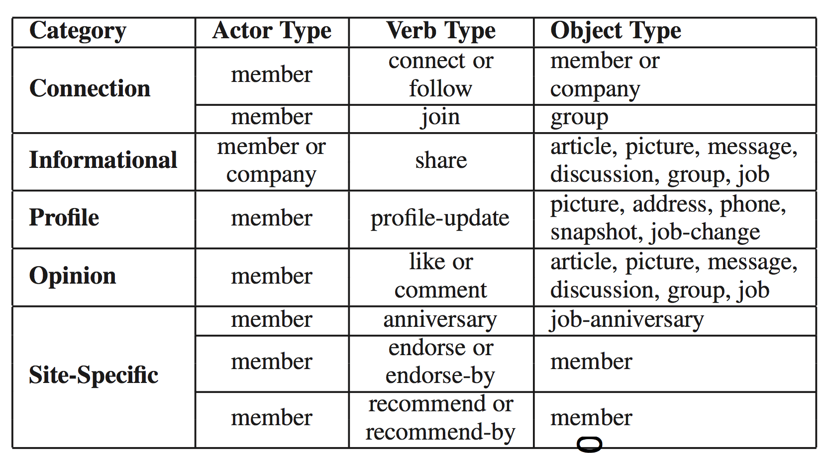
Table 1: A taxonomy of (actor, verb, object) triplets.

In some cases there are nested activities, for example: actor 1 shares an update and actor 2 shares the update of actor 1. In this case we say that the object of the second activity is the first activity, but the root object of the second activity is the object of the first activity.

Taxonomy of Features

Features in the feature vector  are classified into the following categories:

1. viewer-only features : for example, features capturing viewer profile;
2. activity-only features : features capturing activity type, actor type, verb type, update created time, activity impression time, FPR^[2] identity, FPR score, feed position;
3. viewer-actor features : features capturing interaction between viewer and actor;
4. viewer-activity type features : features capturing interaction between viewer and activity type;
5. viewer-actor-activity type features , features capturing interaction between viewer, actor, and activity type;
6. viewer-object features : features capturing interaction between viewer and the object.

The feature vector is a concatenation of the above sub-vectors:  . Since the logistic regression model features a linear combination of features, we can write the inner product in a decomposed form:

.

Feature design and engineering

One limitation of logistic regression is that it estimates probability based on a linear combination of features. Intuitively, it implies that logistic regression models capture a binary click vs no-click relationships where feature vectors corresponding to clicks are linearly separated from feature vectors corresponding to no-clicks.^[3]

An easy way to bypass this limitation is to transform some features through a nonlinear transformation, and then linearly combine the transformed features. This allows building models that capture complex non-linear dependencies between the features and the response using the simple logistic regression model.

Popular feature transformations used by the feed relevance team include:

1. log function on raw counts,
2. indicator function on raw counts,
3. bucketize a numerical feature as a set of categorical features concatenated as a binary sub-vector,
4. linear spline interpolation to fit a set of piecewise linear functions,
5. non-linear function of multiple features, for example product of two functions
6. additional non-linear math functions on raw counts.

Some specific examples of activity only features  are: activityType, verbType, actorType, FPR nameFPR score, update age, bucketized update age, verbTypeage.

Some of the feature groups above are very high dimensional, for example viewer-actor-activity-type affinity or viewer-content affinity. To simplify the engineering and reduce serving latency, we pre-compute these features periodically and store them offline.

The following figure shows the increase in CTR resulting from adding different feature groups.

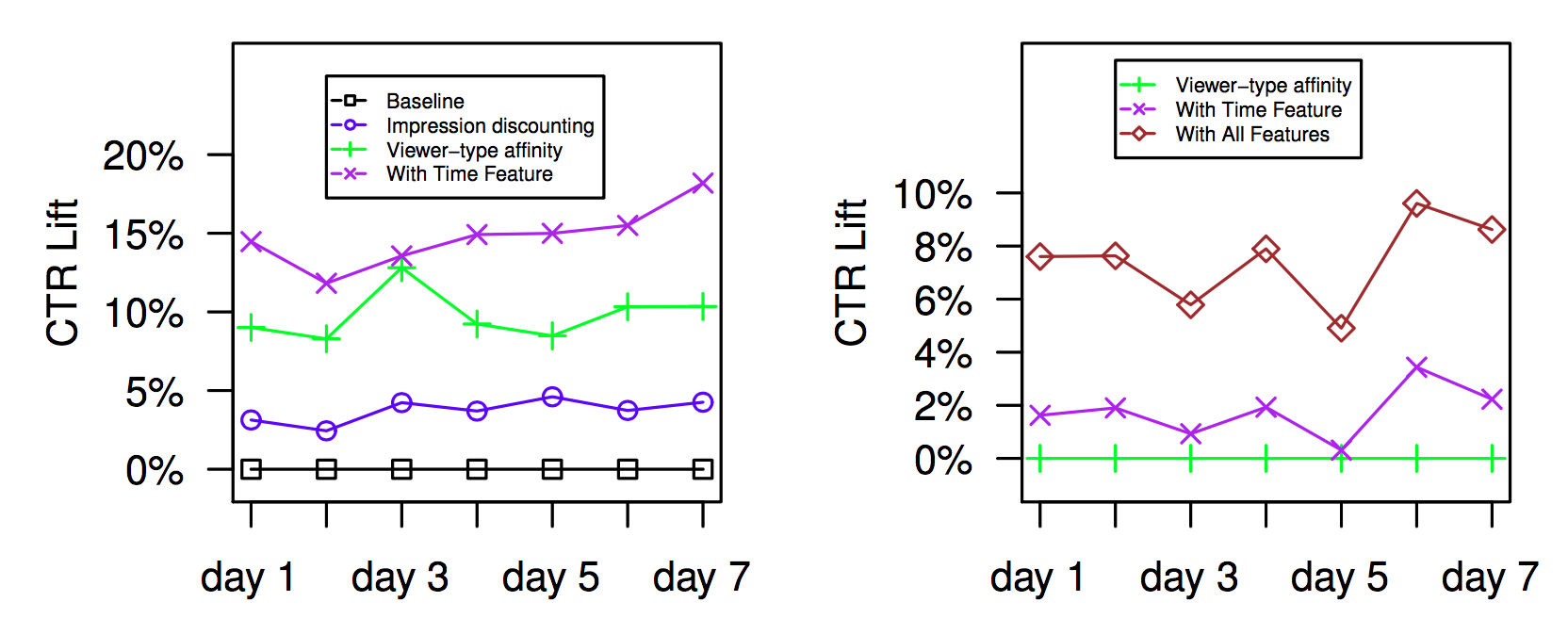
Figure 5: CTR lift of different feature groups over a simple baseline model. Left panel shows CTR increase resulting from adding viewer-type affinity and time features and right panel shows additional CTR increase resulting from adding viewer-type affinity features and all features. Figure originally appeared in the feed relevance KDD 2014 paper (see paper for more details).

References