As a way to encourage engineers to work on interesting problems and try out new technology, LinkedIn Engineering holds an internal coding competition every few months. The winner receives a nice prize, bragging rights, and the privilege of setting up the next contest. In this post, I'll tell you about the 3-colorability graph puzzle and compare solutions in Haskell, C++ and Java.
Graph coloring
Our first engineering-wide competition was to come up with an efficient solver for a graph coloring with 3 colors:

Given an undirected graph, does there exist a way to color the nodes red, green, and blue so that no adjacent nodes have the same color?
Deciding if a graph admits a k-coloring for k > 2 is known to be NP complete. Some of the competitors implemented solutions from research papers that were shown to have very good characteristics against difficult graphs. Other people tried variations on a greedy algorithm with backtracking logic. These usually also had some level of optimization for known graph types.
Solutions were submitted in a number of languages. Today, we'll focus on three of them to get a good look at the variety of possible approaches and compare the top performers (click the links to see the code): Haskell, C++ and Java.
Haskell
One team used Haskell to implement the algorithm found in "3-Coloring in Time O(1.3289^n)". Specifically, the solution implemented covered the CSP transform and the CSP algorithm. It did not cover the graph preprocessing simplification steps. Getting the algorithm to work correctly proved to be very time consuming. By the time they got it working, the team only had time to try a few simple unit tests before submitting. You can play around with the code here.
Java
The Java team used a primarily greedy algorithm with backtracking. It emphasized minimal memory and byte code size. It used two threads, one working in presented graph order and the other working in an order determined by the number of edges. The team wrote a test suite that included several hand coded graphs that they knew in advance were colorable or not as well as code to generate some larger, solvable graphs. Take a look at the code here.
C++
The C++ team implemented a greedy algorithm with backtracking. It would start with the 3-clique with the highest total vertex count, default to the single node with the highest vertex count if it could find no 3-cliques and mark bordering nodes as not colorable a given color as it went. The greedy algorithm would order based on 1) minimal possible color possibilities, 2) vertex count and lastly (3) based on the file order. It also had a background thread that looked for all the 3-cliques and checked if the forced coloring for a 3-clique caused a non-colorable graph. This caught both 4-cliques and various odd numbered wheel graphs, which are not 3 colorable. The C++ code can be found here.
The first implementation used recursion, which allowed for easy backtracking. The team also wrote a suite of basic test cases, including a 4-clique, 5-wheel graph, a 6-wheel graph, an empty graph, some unconnected nodes, a band, and a line. After these were all working, some tools were downloaded for generating large random graphs. The larger such random graphs (250K+ nodes) exposed a stack overflow problem. It was necessary to switch from a recursive implementation to a finite state machine (FSM) to represent attempted coloring.
Since the first pass was not tail recursive, the conversion to a FSM was challenging, especially for the backtracking portion. The team tried a dozen hand-coded graphs and almost 50 randomly generated tests, but none of them ever executed the backtrack code. Every graph in the test suite could either be solved greedily or could be proved to be non-solvable by containing an odd-wheel graph.
Generating hard graphs
The problem then became to generate "hard" graphs. Given the problem is NP-complete, they decided to look at converting a known hard problem to a 3-colorable graph problem. One of the easier problems to use for this conversion was 3-CNFSat. The team wrote a script to convert any 3-CNFSat statement in to a 3-colorability graph. A simple example of this conversion would be:
Visually (!A|B|C) would converted to :-
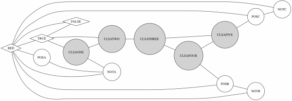
A slightly more complicated example (!A|B|C) & (!A|!B|!C) as a file conversion would become:-
RED:TRUE,FALSE,POSA,NOTA,POSB,NOTB,POSC,NOTC
FALSE:RED,TRUE
TRUE:RED,FALSE,CLSAONE,CLSATWO,CLSBONE,CLSBTWO
CLSAONE:TRUE,CLSATWO,NOTA
CLSATWO:TRUE,CLSAONE,CLSATHREE
CLSATHREE:CLSATWO,CLSAFOUR,CLSAFIVE
CLSAFOUR:CLSATHREE,CLSAFIVE,POSB
CLSAFIVE:CLSATHREE,CLSAFOUR,POSC
CLSBONE:TRUE,CLSBTWO,NOTA
CLSBTWO:TRUE,CLSBONE,CLSBTHREE
CLSBTHREE:CLSBTWO,CLSBFOUR,CLSBFIVE
CLSBFOUR:CLSBTHREE,CLSBFIVE,NOTB
CLSBFIVE:CLSBTHREE,CLSBFOUR,NOTC
POSA:RED,NOTA
NOTA:RED,POSA,CLSAONE,CLSBONE
POSB:RED,NOTB,CLSAFOUR
NOTB:RED,POSB
POSC:RED,NOTC,CLSAFIVE
NOTC:RED,POSC,CLSBFIVE
Value nodes are prefixed with either POS or NOT to provide a namespace and prevent collisions with any of the meta nodes this conversion introduces. This successfully generated "hard" graphs that executed the backtrack code in the C++ solution and allowed the team to find and fix a few bugs in their FSM.
The results
We tested the 3 solutions on a Mac tower running Ubuntu with 40GB of RAM and two 4-core 2.27GHz Xeon processors. We ran them against a number of different graphs: the test cases can be found here.
Theoretically, with a worst-case run-time of O(1.32^n), we expected the Haskell solution to outperform the two other solutions, which used O(2.45^n) greedy algorithms. In reality, the Haskell team stumbled out of the gate: on small graphs, performance was poor, possibly due to some sort of Haskell overhead. For the larger graphs, the implementation tended to run out of memory or hit stack overflows. Perhaps if they had more time and test code, they could've caught these problems earlier, but as it is, the Haskell code lagged far behind the Java and C++ solutions, which are so much faster that they are barely visible on this chart:
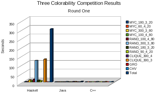
To get a better look at the Java and C++ solutions, we remove Haskell from the graph and zoom in:
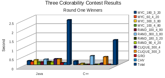
The times for these two programs were within a standard deviation, so we decided to hold a sudden death round to decide the final winner. Each team was asked to create two new problems to be used in the final competition. One problem would need to be solvable, while the other problem should not be solvable. For the C++ team this was relatively easy, because their test script was able to generate arbitrarily hard graphs.
At this time, we discovered that the ordering of the nodes in the input file greatly affected the performance. It was possible to order the graphs to allow the greedy algorithm to work efficiently (for instance by putting NOTA before POSA in this example). However, the decision was made to keep the ordering difficult. They then added a 5-wheel to a 20K hard graph to generate the impossible case. Here are the results:

From this final round, we picked the C++ solution as the winner. It's total time was 40% faster than Java. Moreover, whereas the Java solution violated the 5 minute limit on two of its runs, the C++ solution broke the 5 minute barrier only once.
A few lessons
Whether you prefer Haskell, C++ or Java, the key lesson to take away is that thorough testing is king. The very limited testing of the Haskell solution meant that it did not hold up well against even basic cases. The Java solution did well on basic cases and some large graphs, but their test cases omitted small graphs that were hard to solve. The C++ team had the most thorough testing solution and prevailed.
There are many different ways to implement a solution and even the best algorithm can fail without proper testing. For that matter, there are also many different ways to test and shallow testing can create a false sense of security. A deep understanding of the problem is essential to ensuring the relevant parts of the problem space are tested; code coverage tools are essential to ensuring that the relevant parts of the implementation are tested.
A second lesson is that testing and developing solutions in different languages and different environments involves its own unique set of challenges. For example, the C++ implementation was built using the GNU Compiler Collection (GCC) on Mac OSX. However, the official test system was a Fedora Linux box. On competition day, several hours were lost resolving differences in the GCC flag syntax and Posix thread libraries. Even the Java solution had issues on different computers: on one, the same graph took 30 minutes; on another, just 2. OS, drivers, code and most of the hardware were identical. The only difference we found was that one box had half the L3 cache of the other. In other words: take all benchmarks with a grain of salt.
Try it yourself!
If you wish to experiment with the graph colorability problem yourself, help yourself to the code: